(Adopted from MIT 6.S191)

🌌 Latent Variable Models & Autoencoders: Learning the Hidden Causes of Data

---

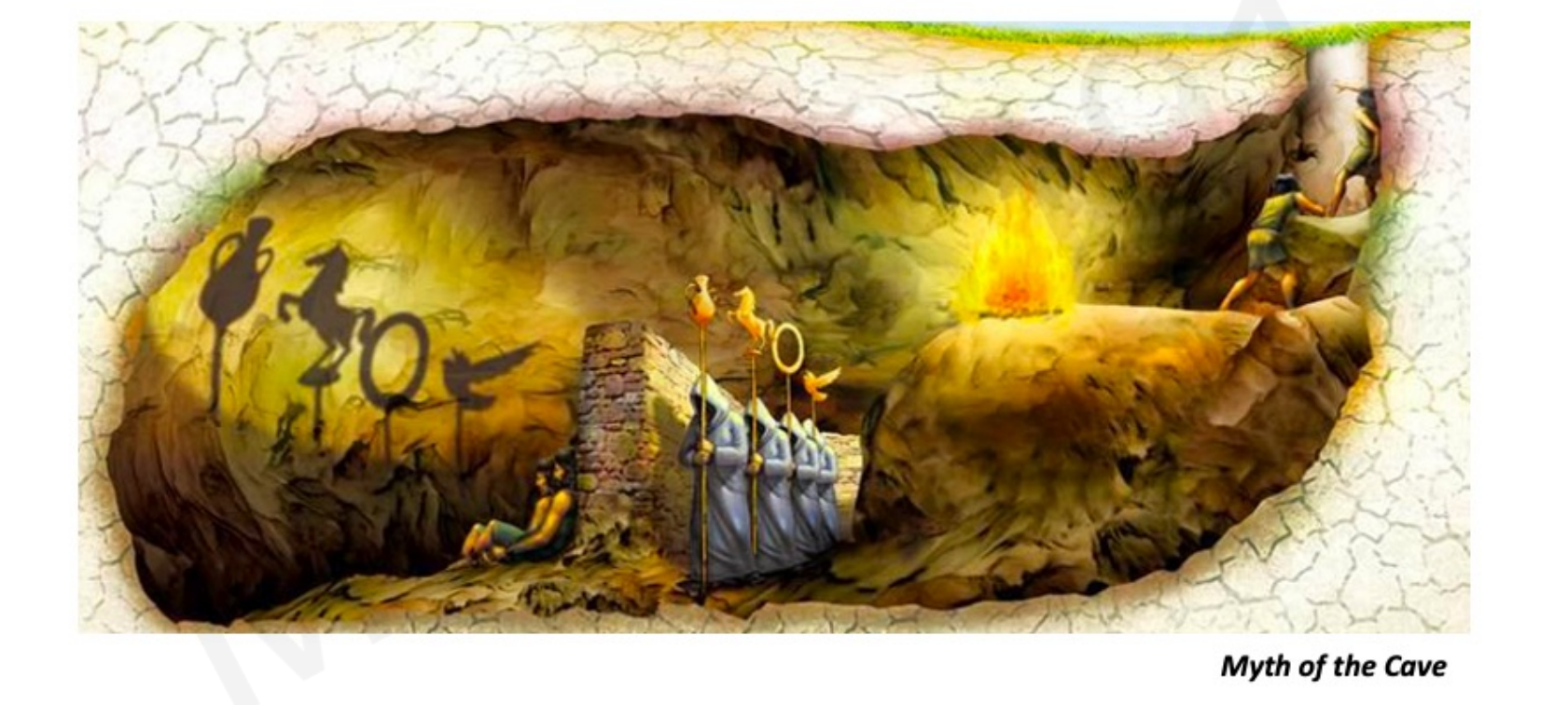
🔮 Introduction: What We See vs. What’s Hidden

Think about handwriting. When you see a digit like “7,” you see 784 pixels (28×28 image). But beneath the pixels are hidden factors:

• the identity of the digit,
• the angle of writing,
• the pen thickness,
• the writer’s style.

These hidden factors are latent variables — they’re not directly observed, but they generate the data we see.

👉 Latent Variable Models (LVMs) are about discovering these hidden causes. They are the foundation of Generative AI, because they let us understand, compress, and create data.

---

🎯 Supervised vs. Unsupervised Learning

Before diving deeper, let’s place LVMs in the ML landscape.

• Supervised learning: you get input–output pairs $(x,y)$. Example: predict house price given size & location.
• Unsupervised learning: you only have inputs $x$. Example: discover that some houses cluster into “luxury” vs “budget.”

Latent variable models live in the unsupervised world. They don’t just cluster; they explain data with hidden variables that we can’t see but can infer.

---

🌀 Generative Modeling: The Mathematical View

A generative model learns how data is produced. Instead of just saying “this is a 7,” it asks: what hidden variables caused this 7 to look this way?

Formally:

• $z$: latent variables (hidden causes).
• $p(z)$: prior distribution over latent space (often Gaussian).
• $p(x|z)$: likelihood of observing data $x$ given latent $z$.

By modeling this, we can:

• Debias: remove unwanted hidden factors (like gender in embeddings).
• Detect anomalies: data that doesn’t fit the latent structure stands out.
• Generate new samples: by sampling a new $z$ and decoding it.

---

🧩 Autoencoders: A Practical Latent Variable Model

The Autoencoder (AE) is one of the simplest ways to learn latent representations.

How It Works

• Encoder: squashes input $x$ into a low-dimensional code $z$.
• Decoder: tries to reconstruct $\hat{x}$ from $z$.
• Loss: minimize reconstruction error.

The bottleneck forces the network to learn a compressed representation. If it can reconstruct well, then $z$ must capture the important patterns in $x$.

---

🔍 Intuition: Autoencoder as Nonlinear PCA

• PCA reduces dimensionality by finding the most “important” directions.
• Autoencoders do the same but nonlinearly.
• This means they can capture curved manifolds (like digit shapes), not just straight directions.

---

🛠️ Building an Autoencoder in PyTorch

Let’s train an AE on MNIST:

import torch
import torch.nn as nn
import torch.optim as optim
from torchvision import datasets, transforms
from torch.utils.data import DataLoader

# Dataset
transform = transforms.ToTensor()
train_data = datasets.MNIST(root="./data", train=True, download=True, transform=transform)
train_loader = DataLoader(train_data, batch_size=128, shuffle=True)

# Autoencoder Model
class Autoencoder(nn.Module):
    def __init__(self):
        super().__init__()
        self.encoder = nn.Sequential(
            nn.Flatten(),
            nn.Linear(784, 128), nn.ReLU(),
            nn.Linear(128, 32)   # latent code
        )
        self.decoder = nn.Sequential(
            nn.Linear(32, 128), nn.ReLU(),
            nn.Linear(128, 784), nn.Sigmoid()
        )
    def forward(self, x):
        z = self.encoder(x)
        x_hat = self.decoder(z)
        return x_hat.view(-1, 1, 28, 28), z

model = Autoencoder()
optimizer = optim.Adam(model.parameters(), lr=1e-3)
criterion = nn.MSELoss()

# Training loop
for epoch in range(5):
    for x, _ in train_loader:
        x_hat, _ = model(x)
        loss = criterion(x_hat, x)
        optimizer.zero_grad()
        loss.backward()
        optimizer.step()
    print(f"Epoch {epoch+1}, Loss={loss.item():.4f}")

---

🎨 Visualizing the Latent Space

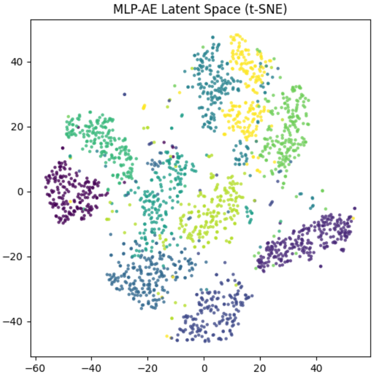
Once trained, the encoder maps digits into a latent space. Let’s see what it looks like with t-SNE:

from sklearn.manifold import TSNE
import matplotlib.pyplot as plt

latents, labels = [], []
model.eval()
with torch.no_grad():
    for x, y in train_loader:
        _, z = model(x)
        latents.append(z)
        labels.append(y)

import numpy as np
latents = torch.cat(latents).numpy()
labels = torch.cat(labels).numpy()

z2d = TSNE(n_components=2).fit_transform(latents)
plt.scatter(z2d[:,0], z2d[:,1], c=labels, cmap="tab10", s=5)
plt.colorbar()
plt.title("Latent Space Visualization (MNIST Autoencoder)")
plt.show()

👉 You’ll see clusters: all “3”s are near each other, “7”s cluster separately. The AE has discovered structure without labels!

---

⚡ Can Autoencoders Generate New Data?

This is where things get tricky.

We might try:

with torch.no_grad():
    z = torch.randn(16, 32)  # random latent samples
    samples = model.decoder(z).view(-1,1,28,28)

But usually, the results look blurry or meaningless.

---

😬 The Problem: Why Autoencoders Struggle

Autoencoders are trained only to reconstruct data they’ve seen. They don’t learn a nice, smooth latent distribution.

• Encoder maps real inputs into some weird shape in latent space.
• If we sample random $z$ outside that shape, the decoder has no idea what to do.

So while AEs are excellent compressors, they’re poor generators.

---

🔑 Enter Variational Autoencoders (VAEs)

To fix this, VAEs make the latent space probabilistic.

• Encoder outputs a distribution (mean & variance).
• A regularization term (KL divergence) pushes latent codes toward a Gaussian.

This way, random samples from $\mathcal{N}(0,1)$ decode into realistic data. 👉 VAEs are true generative models, unlike vanilla AEs.

---

🌟 Applications of Autoencoders

• Dimensionality reduction: nonlinear PCA.
• Anomaly detection: high reconstruction error = anomaly.
• Image denoising: train with noisy inputs, reconstruct clean outputs.
• Feature extraction: latent vectors as embeddings.

---

✅ Conclusion

Latent Variable Models let us peek beneath the surface of data.

• Autoencoders give us a practical way to learn compressed, meaningful codes.
• They reconstruct well but struggle with generation.
• VAEs (and later GANs, Diffusion Models) build on this idea to generate new, realistic samples.

👉 Think of Autoencoders as microscopes: they help us see the hidden structure. 👉 But if we want to create, we need probabilistic LVMs like VAEs.

---

\