Exploring the Foundations of Computer Vision: From Pixels to Feature Points

Computer Vision is a fascinating field that enables computers to “see” and interpret the world from digital images and videos. At its core, it’s about making sense of high-dimensional data, transforming raw visual information into meaningful insights. This blog post will take you through some fundamental concepts, including what an image is, how we process it through filtering, detect important features like edges and corners, and understand the implications of sampling.

What is an Image? The Digital Canvas

At a fundamental level, an image is a signal. More specifically, it’s a multi-dimensional function that contains information about a phenomenon. Think of light hitting a camera sensor; this continuous signal is then converted into a discrete one through a process called sampling.

In a digital image, this sampling results in a grid of pixels (picture elements). Each pixel stores an intensity or ‘brightness’ value. When capturing an image, an analog signal is converted into discrete numerical values, a process known as quantization. The number of bits used for quantization (bit depth) affects the radiometric resolution, determining how many distinct brightness levels can be represented.

For example, an 8-bit grayscale image means each pixel can have 256 different intensity values (from 0 to 255).

Images in Python

In Python, an image can be represented as a NumPy array. A grayscale image is typically a 2D array (N x M), where im[y, x] gives the pixel value at row y and column x.

import numpy as np
import matplotlib.pyplot as plt
import cv2

# Load the image from file (replace with your cat image path)
image_array = cv2.imread('example.jpg', cv2.IMREAD_GRAYSCALE)  # Loads as grayscale

print(f'First pixel: {image_array[0,0]}')
plt.imshow(image_array, cmap='gray')
plt.title("Example Grayscale Image")
plt.axis('off')
plt.show()

First pixel: 40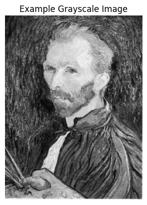

Image Filtering: Modifying Signals

Filtering is an operation that modifies a signal. In image processing, filters are used for various purposes, such as removing undesirable components (e.g., noise), transforming the signal in a desired way, or extracting specific components.

A common type of filter is the linear filter, which exhibits properties like linearity and shift/translation invariance. Any linear, shift-invariant operator can be represented as a convolution. This operation involves sliding a small matrix, called a kernel (or filter), over the image and computing a function of the local neighborhood at each position.

A simple example of a 1D filter is a moving average, which smooths out data by averaging values within a defined window size k. In 2D, a box filter is a basic example where each pixel is replaced by the average of its neighbors within a square kernel.

Python for Image Filtering (Conceptual)

While a full convolution implementation is complex, here’s a conceptual idea for a simple 2D filtering operation:

# Example 3x3 Box Filter (averaging kernel)
box_filter_kernel = np.ones((3, 3), np.float32) / 9.0

# Apply the filter using cv2
filtered_image = cv2.filter2D(image_array, -1, box_filter_kernel)

print("\nFiltered Image (conceptual):\n", filtered_image)
plt.imshow(filtered_image, cmap='gray')
plt.title("Example Filtered Image (Box Filter)")
plt.axis('off')
plt.show()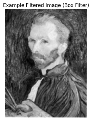

Edge Detection: Finding Discontinuities

Edge detection is the process of identifying parts of a digital image where there are sharp changes or discontinuities in image intensity. Edges are crucial for various computer vision tasks, including recognizing objects and reconstructing scenes.

Edges can be caused by various factors, such as changes in surface orientation, depth, color, or illumination. A common approach to detect edges is by finding the gradient of the image intensity function; edges typically correspond to the extrema (peaks) of this derivative.

Noise in an image can severely affect derivative calculations, making it harder to find true edges. To mitigate this, a smoothing filter (like a Gaussian filter) is often applied before computing derivatives. This introduces a “smoothing-localization tradeoff”: more smoothing reduces noise but blurs the edges.

Python for Edge Detection (Conceptual)

Edge detection often involves applying derivative filters, such as the Sobel operator.

# Sobel edge detection using cv2
sobel_x = cv2.Sobel(image_array, cv2.CV_64F, 1, 0, ksize=3)
sobel_y = cv2.Sobel(image_array, cv2.CV_64F, 0, 1, ksize=3)

sobel_combined = cv2.magnitude(sobel_x, sobel_y)
sobel_combined = np.uint8(np.clip(sobel_combined, 0, 255))

plt.imshow(sobel_combined, cmap='gray')
plt.title("Example Edge Detection (Sobel Filter)")
plt.axis('off')
plt.show()

(Visualization would show the outlines of objects or significant intensity changes in the image.)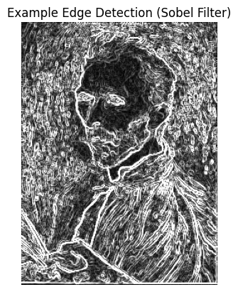

Sampling and Aliasing: The Pitfalls of Resolution

When creating lower-resolution images, we often subsample by discarding rows and columns. This process can lead to an undesirable artifact called aliasing. Aliasing occurs when two different signals become indistinguishable from each other because the sampling rate is too low. Essentially, there aren’t “enough samples” to accurately represent the original signal.

The Nyquist-Shannon Sampling Theorem states that to perfectly reconstruct a continuous signal from its samples, the sampling frequency must be at least twice the maximum frequency present in the original signal. If this condition is not met, aliasing will occur.

To prevent aliasing during downsampling, a technique called anti-aliasing is used. This involves applying a low-pass filter (which blurs the image) to remove high frequencies before subsampling.

Python for Downsampling with Anti-aliasing (Conceptual)

# Downsample without anti-aliasing (will likely show aliasing)
low_res_image_aliased = image_array[::2, ::2]  # Subsample every other pixel

# Downsample with anti-aliasing using GaussianBlur from cv2
blurred_image = cv2.GaussianBlur(image_array, (5, 5), sigmaX=1)
low_res_image_anti_aliased = blurred_image[::2, ::2]

plt.figure(figsize=(10, 5))
plt.subplot(1, 2, 1)
plt.imshow(low_res_image_aliased, cmap='gray')
plt.title("Downsampled with Aliasing")
plt.axis('off')
plt.subplot(1, 2, 2)
plt.imshow(low_res_image_anti_aliased, cmap='gray')
plt.title("Downsampled with Anti-aliasing")
plt.axis('off')
plt.show()

(Visualizations would clearly show the difference in quality, with aliased images exhibiting jagged or Moiré patterns.)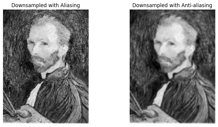

Interest Points & Feature Descriptors: Anchors for Understanding

Beyond edges, computer vision often relies on interest points, also known as corners, key points, or local features. These are specific, distinct points in an image that are robust to changes in viewpoint, lighting, and other transformations.

The ability to find correspondence (matching points or regions across multiple images) is fundamental to many applications. These applications include:

• Image alignment
• 3D reconstruction
• Motion tracking
• Object recognition
• Panorama stitching

A good feature detector aims for:

• Distinctiveness: Each detected point should be unique enough to be reliably matched.
• Repeatability: The detector should consistently find the same points in different views of the same scene, even under geometric (e.g., rotation) or photometric (e.g., brightness) variations.
• Compactness and Efficiency: The representation of these features should be small and allow for fast matching.

The Harris corner detector is a classic algorithm used for identifying such interest points.

Python for Feature Points (Conceptual)

Libraries like OpenCV are commonly used for detecting feature points.

# Harris Corner Detection using cv2
img_cv = np.copy(blurred_image)
img_cv = np.float32(img_cv)

dst = cv2.cornerHarris(img_cv, blockSize=2, ksize=3, k=0.04)
dst = cv2.dilate(dst, None)

# Create a color image to mark corners in red
img_color = cv2.cvtColor(blurred_image, cv2.COLOR_GRAY2BGR)
img_color[dst > 0.03 * dst.max()] = [0, 0, 255]  # Mark corners in red

plt.imshow(cv2.cvtColor(img_color, cv2.COLOR_BGR2RGB))
plt.title("Harris Corner Detection")
plt.axis('off')
plt.show()

(A visualization would highlight detected corners on an image.)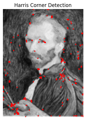

Conclusion

Understanding these fundamental concepts – from how an image is formed digitally to applying filters, detecting edges, managing sampling issues, and identifying key feature points – provides a strong foundation for delving deeper into the exciting world of computer vision. These building blocks are essential for developing more complex algorithms that enable machines to perceive and interact with visual information, just like humans do.