PyTorch Primer

PyTorch Fundamentals: A Deep Dive into Tensors and Efficient Computation

PyTorch is a powerful deep learning framework that provides flexibility and speed for building and training neural networks. This tutorial will explore some fundamental PyTorch concepts, focusing on tensors, memory and compute accounting, and essential tensor operations, drawing insights from a Stanford CS336 lecture.

1. The Building Blocks: Tensors

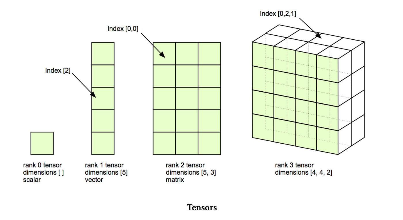
At the core of PyTorch, and indeed deep learning, are tensors. Tensors are multi-dimensional arrays used to store all types of data: parameters, gradients, optimizer states, input data, and activations.

1.1 Tensors vs. NumPy Arrays: A Comparison

If you’re familiar with Python’s scientific computing stack, you’ve likely used NumPy arrays. PyTorch tensors are very similar to NumPy arrays in terms of their API and functionality for numerical operations. Both support operations like slicing, reshaping, and element-wise arithmetic.

import torch
import numpy as np

# NumPy array
np_array = np.array([[1., 2.], [3., 4.]])
print(f"NumPy array:\n{np_array}")

# PyTorch tensor from NumPy array
torch_tensor_from_np = torch.from_numpy(np_array)
print(f"PyTorch tensor from NumPy:\n{torch_tensor_from_np}")

# Convert PyTorch tensor back to NumPy array
np_array_from_torch = torch_tensor_from_np.numpy()
print(f"NumPy array from PyTorch:\n{np_array_from_torch}")

# Element-wise addition
a_np = np.array([1, 2, 3])
b_np = np.array([4, 5, 6])
c_np = a_np + b_np
print(f"NumPy element-wise addition: {c_np}")

a_torch = torch.tensor([1, 2, 3])
b_torch = torch.tensor([4, 5, 6])
c_torch = a_torch + b_torch
print(f"PyTorch element-wise addition: {c_torch}")

Key Differences:

1. GPU Acceleration: This is the most significant difference. PyTorch tensors can be easily moved to and operated on GPUs, providing massive speedups for deep learning computations. NumPy arrays are strictly CPU-bound.

2. Automatic Differentiation (Autograd): PyTorch tensors have built-in support for automatic differentiation, a crucial feature for training neural networks. This allows PyTorch to automatically compute gradients of operations, which are then used in optimization algorithms like stochastic gradient descent. NumPy has no built-in autograd functionality.

   import torch
   
   x = torch.tensor(2.0, requires_grad=True) # Tell PyTorch to track gradients for x
   y = x**2 + 5
   z = y * 3
   
   z.backward() # Compute gradients
   print(f"Gradient of z with respect to x: {x.grad}") # Should be 12.0 (dz/dx = d(3*(x^2+5))/dx = 6x)

   NumPy does not have an equivalent requires_grad=True or .backward() method.

3. Dynamic Computation Graph: PyTorch uses a dynamic computation graph (also known as “define-by-run”). This means the computation graph is built on the fly as operations are performed. This flexibility makes debugging easier and allows for variable input sizes or conditional logic within the model. TensorFlow (until Eager Execution was default) traditionally used static graphs, which were compiled before execution.

1.2 Creating Tensors

You can create tensors in various ways. By default, PyTorch tensors are stored on the CPU.

import torch

# Create a 4x8 tensor with default float32 data type
x = torch.zeros(4, 8)
print(f"Tensor x:\n{x}")
print(f"Data type of x: {x.dtype}")
print(f"Shape of x: {x.shape}")

# Create an uninitialized tensor
y = torch.empty(2, 2)
print(f"Uninitialized tensor y:\n{y}")

1.3 Memory Accounting with Tensors

Understanding memory usage is crucial for efficiency. The memory a tensor consumes depends on the number of elements and the data type of each element.

Floating-point numbers are the primary way tensors store values. Different precision levels exist:

• Float32 (FP32): The default “single precision,” using 32 bits (4 bytes) per value. It’s considered the gold standard in computing and is generally safe for training, though it requires more memory.

  # Memory usage example for a 4x8 float32 matrix
  rows, cols = 4, 8
  num_elements = rows * cols
  element_size_bytes = 4 # for float32 (32 bits)
  memory_usage = num_elements * element_size_bytes
  print(f"Memory usage for a {rows}x{cols} float32 tensor: {memory_usage} bytes")

• Float16 (FP16): “Half precision,” using 16 bits per value. It halves memory usage and can speed up computations. However, its limited dynamic range can lead to underflow (numbers rounding to zero) or overflow, especially in large models, causing instability. It’s generally not recommended for deep learning training at this point.

• BFloat16 (BF16): “Brain float,” also 16 bits, developed to address FP16’s dynamic range issues. It allocates more bits to the exponent (like FP32) and fewer to the fraction (like FP16). This provides a dynamic range similar to FP32 while using FP16’s memory footprint, making it suitable for many computations in deep learning. For optimizer states and parameters, Float32 is often still needed for training stability.

• FP8 (8-bit float): Developed more recently (2022 by Nvidia), it uses 8 bits per value, offering even faster computation and less memory. It’s supported by newer hardware like the H100.

For optimal efficiency, “mixed precision training” is often used, where different precisions are applied at various stages of the pipeline (e.g., Float32 for attention, BF16 for matrix multiplications).

1.4 How Tensors Are Stored in Memory: Data Pointer, Size, and Strides

PyTorch tensors, like NumPy arrays, are abstractions over a contiguous block of memory. Each tensor object holds key metadata that describes how to interpret this memory block:

1. Data Pointer: This is the memory address of the first element of the underlying data storage. All elements of the tensor are stored sequentially from this address.
2. Size (Shape): This tuple defines the logical dimensions of the tensor (e.g., $(2, 3)$ for a 2x3 matrix).
3. Strides: This is the crucial part for understanding memory layout. Strides are a tuple of integers indicating the number of elements (or bytes, depending on implementation details, but conceptually elements) you need to skip in the underlying memory block to get to the next element along each dimension.

Let’s illustrate with an example:

import torch

# Create a 2x3 tensor
x = torch.tensor([[1, 2, 3],
                  [4, 5, 6]])
print(f"Tensor x:\n{x}")
print(f"Shape of x: {x.shape}")
print(f"Strides of x: {x.stride()}") # (3, 1) if contiguous
print(f"Is x contiguous? {x.is_contiguous()}") # True

Memory Layout for a Contiguous Tensor:

For x = torch.tensor([[1, 2, 3], [4, 5, 6]]), stored in a contiguous block of memory, the values would be laid out as: [1, 2, 3, 4, 5, 6].

• Shape: $(2, 3)$ (2 rows, 3 columns)
• Strides: $(3, 1)$
  • To move to the next element in the first dimension (next row), you skip 3 elements in memory. (From 1 to 4, you skip 2 and 3).
  • To move to the next element in the second dimension (next column), you skip 1 element in memory. (From 1 to 2, you skip 0 elements, landing directly on the next).

Tensor Views and Non-Contiguous Memory:

When you create a “view” of a tensor (e.g., by slicing or transposing), PyTorch often does not create a new copy of the data. Instead, it creates a new tensor object that points to the same underlying memory block but with updated shape and strides to reflect the new logical arrangement.

import torch

x = torch.tensor([[1, 2, 3], [4, 5, 6]])
print(f"Original tensor x:\n{x}")
print(f"Strides of x: {x.stride()}") # (3, 1)

# Transposing creates a view with different strides
y = x.T # Equivalent to x.transpose(0, 1)
print(f"Transposed view y:\n{y}")
print(f"Strides of y: {y.stride()}") # (1, 3) - notice they are swapped
print(f"Is y contiguous? {y.is_contiguous()}") # False (likely)

# Check if they share the same storage
print(f"Do x and y share storage? {x.storage().data_ptr() == y.storage().data_ptr()}") # True

For y = x.T (which is [[1, 4], [2, 5], [3, 6]]):

• Shape: $(3, 2)$ (3 rows, 2 columns)
• Strides: $(1, 3)$
  • To move to the next element in the first dimension (next row), you skip 1 element in memory (from 1 to 2, from 4 to 5). This is because the original data [1, 2, 3, 4, 5, 6] means the elements for the next row are not directly adjacent anymore after transposition.
  • To move to the next element in the second dimension (next column), you skip 3 elements in memory (from 1 to 4, from 2 to 5).

Why contiguous() is important: Some PyTorch operations (especially those that involve reshaping, like view()) require the tensor to be contiguous in memory. If a tensor is not contiguous, calling .contiguous() will return a new tensor with the data copied into a contiguous memory block. This is an explicit data copy, which can be computationally expensive but necessary for certain operations.

import torch

# Transposing creates a non-contiguous view
y = torch.randn(2, 3).T
print(f"Transposed view y:\n{y}")
print(f"Is y contiguous? {y.is_contiguous()}") # False (likely)

# Calling .contiguous() creates a copy if not contiguous
z = y.contiguous()
print(f"Contiguous copy z:\n{z}")
print(f"Do y and z share storage? {y.storage().data_ptr() == z.storage().data_ptr()}") # False
print(f"Is z contiguous? {z.is_contiguous()}") # True

Conceptual Diagram: Contiguous vs. Non-Contiguous Imagine a 2x3 matrix: [[A, B, C], [D, E, F]]

In memory, if it’s contiguous, it might be stored linearly as [A, B, C, D, E, F]. If you transpose it to a 3x2 matrix: [[A, D], [B, E], [C, F]]

A view of this transposed matrix (y) doesn’t rearrange the underlying [A, B, C, D, E, F] block. Instead, y’s strides tell it how to “jump” through this original block to find its elements (e.g., to get from A to D, it jumps over B and C). This makes it non-contiguous. If you call .contiguous(), PyTorch creates a new block of memory [A, D, B, E, C, F] and copies the data into it, making the new tensor z contiguous.

2. GPU Computation

For deep learning, leveraging GPUs is essential for performance, as they offer orders of magnitude faster computation than CPUs. Tensors are by default on the CPU and must be explicitly moved to the GPU.

import torch

# Create a tensor on CPU
x_cpu = torch.zeros(3, 3)
print(f"x_cpu device: {x_cpu.device}")

# Move tensor to GPU (if CUDA is available)
if torch.cuda.is_available():
    x_gpu = x_cpu.to('cuda')
    print(f"x_gpu device: {x_gpu.device}")
    # You can also create tensors directly on the GPU
    y_gpu = torch.ones(3, 3, device='cuda')
    print(f"y_gpu device: {y_gpu.device}")
else:
    print("CUDA is not available. Running on CPU.")

Conceptual Diagram: CPU to GPU Transfer Visualize a CPU with its own RAM (main memory) and a GPU with its own dedicated memory (HBM). When you create a tensor on the CPU, it resides in the CPU’s RAM. To perform computations on the GPU, the tensor data must be explicitly copied from CPU RAM to GPU HBM. This data transfer takes time and is a factor in overall efficiency.

3. Essential Tensor Operations

3.1 Matrix Multiplications (MatMuls)

Matrix multiplication is the “bread and butter of deep learning” and is generally the most expensive operation for large enough matrices.

For a matrix multiplication of an $(M \times N)$ matrix with an $(N \times P)$ matrix, resulting in an $(M \times P)$ matrix, the number of floating-point operations (FLOPs) is approximately $2 \times M \times N \times P$.

In deep learning, operations are often batched. For example, in language models, you might have tensors with dimensions like (Batch Size, Sequence Length, Feature Dimension). PyTorch handles batching gracefully for matrix multiplications.

import torch

# Simple matrix multiplication
matrix_a = torch.randn(16, 32)
matrix_b = torch.randn(32, 2)
result = matrix_a @ matrix_b # or torch.matmul(matrix_a, matrix_b)
print(f"Shape of result: {result.shape}")

# Batched matrix multiplication
batch_size = 4
sequence_length = 10
hidden_dim_in = 64
hidden_dim_out = 128

batched_input = torch.randn(batch_size, sequence_length, hidden_dim_in)
weight_matrix = torch.randn(hidden_dim_in, hidden_dim_out)

# PyTorch automatically handles batch and sequence dimensions
batched_output = batched_input @ weight_matrix
print(f"Shape of batched output: {batched_output.shape}")

3.2 EinSum: Einstein Summation for Tensor Operations

torch.einsum (inspired by Einstein’s summation notation) provides a powerful and readable way to perform various tensor operations, including matrix multiplications, transpositions, and element-wise products, by explicitly naming dimensions. This helps avoid confusion with arbitrary dimension indices like -1 or -2.

Basic Matrix Multiplication with EinSum

import torch

# Equivalent to torch.matmul(A, B)
A = torch.randn(2, 3) # Example: A = (rows, cols)
B = torch.randn(3, 4) # Example: B = (cols, new_cols)

# i, j, k are named dimensions
# j is summed over (common dimension in multiplication)
# i and k appear in the output
C = torch.einsum("ij,jk->ik", A, B)
print(f"EinSum for matrix multiplication result:\n{C.shape}")

Batched Matrix Multiplication with EinSum

import torch

batch = 2
seq_len_1 = 5
seq_len_2 = 7
hidden_dim = 8

X = torch.randn(batch, seq_len_1, hidden_dim) # "bsh" (batch, sequence, hidden)
Y = torch.randn(batch, seq_len_2, hidden_dim) # "bth" (batch, sequence, hidden)

# Dot product for each (batch, sequence_1, sequence_2) pair, summing over hidden_dim
# This could be for attention scores: "bsh,bth->bst"
result = torch.einsum("bsh,bth->bst", X, Y)
print(f"EinSum for batched operation (e.g., attention scores) result:\n{result.shape}")

Reduction with EinSum To sum over a dimension (like mean() or sum() operations), simply omit the dimension name from the output string.

import torch

tensor = torch.randn(3, 4, 5) # (batch, seq, hidden)

# Sum over the 'hidden' dimension
sum_result = torch.einsum("bsh->bs", tensor)
print(f"EinSum sum result shape: {sum_result.shape}")

Rearrange for Complex Reshaping with EinSum-like Syntax Libraries like einops (which provides rearrange) offer even more elegant ways to reshape tensors where one dimension logically represents multiple dimensions. While einops isn’t a core PyTorch function, it extends the einsum philosophy.

Conceptual Example of Rearrange If you have a tensor (Batch, Sequence, Heads * Hidden_dim_per_head) and you want to split the last dimension into (Heads, Hidden_dim_per_head), rearrange allows you to express this clearly: rearrange(tensor, 'b s (h d) -> b s h d', h=num_heads).

4. Compute Accounting: Understanding FLOPs

FLOPs (Floating Point Operations) (lowercase ‘s’) refers to the number of computational operations performed, measuring the amount of computation. FLOPs/second (uppercase ‘S’ or /s) refers to floating-point operations per second, measuring the speed of hardware.

High-end GPUs like the NVIDIA H100 can achieve massive FLOPs/second, but their actual performance depends significantly on the data type (FP32, FP16, BF16, FP8) and whether sparsity is leveraged. Training large models like GPT-3 and GPT-4 requires immense computational power, measured in ExaFLOPs ($10^{18}$ FLOPs).

For most deep learning models, matrix multiplications dominate the computational cost. Therefore, napkin-math estimates of training time often focus primarily on these operations. For a simple linear model, the forward pass FLOPs can be approximated as $2 \times (\text{number of data points}) \times (\text{number of parameters})$. This rough generalization also holds for Transformers if the sequence length isn’t too large.

# Example: FLOPs for a linear model's forward pass
B = 64 # Batch size (number of data points)
D = 512 # Input dimension
K = 256 # Output dimension

# A linear model performs matrix multiplication (input @ weight_matrix)
# Input: (B, D), Weight: (D, K), Output: (B, K)
# Flops = 2 * B * D * K (for the matrix multiplication)
flops = 2 * B * D * K
print(f"FLOPs for a linear model forward pass: {flops}")

5. A Simple PyTorch Training Example: Linear Regression

To solidify these concepts, let’s walk through a complete (though simple) training example: linear regression. This demonstrates how tensors, models, loss functions, and optimizers work together.

Scenario: We want to find a linear relationship $y = mx + b$ that best fits some generated data.

import torch
import torch.nn as nn
import torch.optim as optim
import matplotlib.pyplot as plt

# 1. Data Generation
# We'll generate some synthetic data with a known true relationship
# y = 2x + 1 + noise
true_m = 2.0
true_b = 1.0
num_samples = 100

X = torch.randn(num_samples, 1) * 10 # Random X values, scaled
noise = torch.randn(num_samples, 1) * 2 # Add some noise for realism
y_true = true_m * X + true_b + noise

# 2. Define the Model
# In PyTorch, models are defined by inheriting from nn.Module
class LinearRegression(nn.Module):
    def __init__(self):
        super().__init__()
        # nn.Linear creates two parameters: weight (m) and bias (b)
        # It expects input features, output features
        self.linear = nn.Linear(in_features=1, out_features=1)

    def forward(self, x):
        # The forward pass defines how data flows through the model
        return self.linear(x)

# Instantiate the model
model = LinearRegression()
print(f"Initial model parameters (randomly initialized):\nWeight: {model.linear.weight.item():.4f}, Bias: {model.linear.bias.item():.4f}")

# 3. Define Loss Function and Optimizer
# Loss function: Mean Squared Error (MSE) is common for regression
criterion = nn.MSELoss()

# Optimizer: Stochastic Gradient Descent (SGD)
# It will update the model's parameters (weight and bias) to minimize the loss
optimizer = optim.SGD(model.parameters(), lr=0.01) # Learning rate is crucial!

# Move model and data to GPU if available
device = torch.device("cuda" if torch.cuda.is_available() else "cpu")
model.to(device)
X = X.to(device)
y_true = y_true.to(device)

# 4. Training Loop
num_epochs = 500

for epoch in range(num_epochs):
    # Forward pass: Compute predicted y by passing x to the model
    y_pred = model(X)

    # Calculate loss
    loss = criterion(y_pred, y_true)

    # Backward pass: Compute gradients of loss with respect to model parameters
    # This is where PyTorch's autograd system comes into play!
    optimizer.zero_grad() # Clear previous gradients
    loss.backward()       # Compute gradients
    optimizer.step()      # Update parameters using the gradients

    if (epoch + 1) % 50 == 0:
        print(f'Epoch [{epoch+1}/{num_epochs}], Loss: {loss.item():.4f}')

# 5. Evaluation
# Move model back to CPU for plotting (if trained on GPU)
model.to('cpu')
X_cpu = X.to('cpu')
y_true_cpu = y_true.to('cpu')
predicted_values = model(X_cpu).detach().numpy() # .detach() stops gradient tracking, .numpy() converts to NumPy

print(f"\nFinal model parameters:\nWeight: {model.linear.weight.item():.4f}, Bias: {model.linear.bias.item():.4f}")
print(f"True parameters:\nWeight: {true_m:.4f}, Bias: {true_b:.4f}")

# 6. Visualization
plt.figure(figsize=(10, 6))
plt.scatter(X_cpu.numpy(), y_true_cpu.numpy(), label='True Data', alpha=0.7)
plt.plot(X_cpu.numpy(), predicted_values, color='red', label='Learned Regression Line')
plt.xlabel('X')
plt.ylabel('y')
plt.title('Linear Regression with PyTorch')
plt.legend()
plt.grid(True)
plt.show()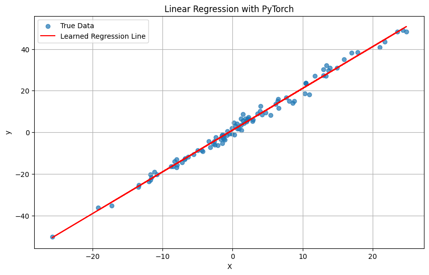

This example clearly shows the flow:

• Data preparation: Tensors X and y_true.
• Model definition (nn.Module): Defines the layers (here, nn.Linear) and the forward pass. The model parameters (weights and biases) are implicitly PyTorch tensors with requires_grad=True.
• Loss function (nn.MSELoss): Quantifies how far off our predictions are.
• Optimizer (optim.SGD): Responsible for updating model parameters based on gradients.
• Training loop:
  • model(X): Forward pass, computes y_pred.
  • criterion(y_pred, y_true): Calculates loss.
  • optimizer.zero_grad(): Crucial step to clear gradients from previous iterations.
  • loss.backward(): The magic of Autograd! It computes dy/dw and dy/db for all parameters.
  • optimizer.step(): Updates w and b using the calculated gradients and the learning rate.

Understanding this simple example provides a solid foundation for tackling more complex neural network architectures in PyTorch.

---

Understanding these fundamental concepts of PyTorch, from tensor representation and its crucial differences from NumPy to efficient computation, advanced operations like EinSum, and the practical application in a training loop, is crucial for building and optimizing deep learning models. Efficiency in deep learning directly translates to reduced costs and faster experimentation cycles.